Peer group comparisons are key elements to our selection process. We always seek to evaluate an asset manager based on his/her ability to deliver better return compare to peers with similar guidelines and constraints over the same time horizon. It is essential for us to assess in an ex-post how skilful the manager is. While it seems an obvious statement, to compare apples with apples, when it comes to asset manager assessments to reach to that result requires to overcome many problems. This article reviews the current approaches used by many, and explores solutions developed by professionals as ourselves to improve the effectiveness of asset manager selection through peer group measures. For the sake of ease, we have based this short paper essentially from a well-documented article published in the CFA Institute Magazine by Antti Raappana, Kimmo Kurki, Fernand Schoppig, and Barry Gillman (the authors) (see below sources).
The most common approach
Is to use peer groups published by data providers. It may provide an assessment against a broad universe of comparison, but as the authors highlighted, there are serious drawbacks such as survivor bias, composition bias, timeliness, and (especially for the broadest peer universes) mismatches against the mandate being measured. Published peer groups can give you an estimate of how well your portfolio has done against competitors with similar benchmarks essentially, but whose mandates may differ from yours, or the population of competitors may not be comprehensive enough.
Using the wrong peer group, or a partial one, gives an inaccurate picture of the true distribution of potential outcomes and might lead to false conclusions on the significance of relative performance.
No suitable peer group exists
For some strategies, a suitable peer group may not even exist. Such is the situation for mandates that combine an “unusual” mix of countries, have constraints in a single country, or have systemic biases in terms of sectors or styles that reduce the peer group universe to few or no peers. However, it is important to distinguish constraints imposed in the mandate or sought after by investors in the fund, from constraints a portfolio manager chooses to introduce on the belief it will improve performance compare to other portfolios with similar benchmark. In the latter, depending on the type of constraints, we would, or not, seek a suitable peer group.
Portfolio Opportunity Distribution
As revealed by the article’s authors, the pioneering work on the first problem was developed by Ron Surz of PPCA, who created portfolio opportunity distributions (PODs)—simulated peer groups comprising all the realistic portfolios that can be constructed from the constituents of a specific index. PPCA publishes PODs that provide peer group comparisons for the US and other developed markets.
The authors have used the ideas behind Ron Surz’s work to solve the second problem: the lack of suitable peer groups for unconventional mandates. The challenge was to develop suitable comparisons where no usable peer groups existed, particularly for specialised small- and mid-cap mandates in regional combinations within the emerging and frontier markets.
They did it by simulating in a model the range of possible portfolio-return outcomes that could have been achieved by following the specific constraints of the selected manager. These constraints included country, market-cap size, number of stocks held, and maximum weight in a stock or sector. Using a Monte Carlo simulation, every randomly generated portfolio with those mandate constraints represented a potential peer portfolio that could have been achieved without stock-selection skills.
By running thousands of simulations to include all the available portfolios that could have been constructed using a particular mandate’s constraints, a comparable peer group portfolio-return distribution can be generated. We could then see how the manager’s actual results over that period compare to that of the generated peer group. This approach also helps in a situation where no appropriate benchmark index is available.
The advantage of these simulations, according to the authors, is that they are tailor-made to the specifics of each manager’s own stated approach, they are not affected by the competing managers whose mandates may not be truly comparable, and it allows for simulated peer groups to be generated for non-standard time periods.
While we agree on the advantages brought by this peer group modelling, in certain circumstances we see some limitation either. For truly active portfolio managers using broad universe of stocks, maintaining high active share and large off-benchmark exposure, (in short, the type of managers we look after in fund selection) the simulation might become complicated to implement. Statistically, the larger the universe of possible stocks to include, the more difficult it is to generate meaningful simulation results.
There’s no commonly accepted set of tools currently available to overcome these problems. As a result, investors, fund selectors and portfolio managers often end up disagreeing over whether the fund’s performance is good or bad given the circumstances and mandate constraints.
The process
The process for a one-period simulation as described by the authors, consists of the five steps below:
- Screen for stocks that fulfill the mandate constraints at the beginning of the period and that have been listed for the full simulation period so that a full-period total return is available. This constitutes the simulation universe.
- Calculate the total return for the period of each stock in the universe.
- Impose portfolio construction constraints (number of stocks, maximum/minimum exposure, country/sector exposure, maximum cash, and any other potential constraints).
- Simulate random portfolios that fulfill those constraints from the eligible stock universe.
- Compare actual portfolio performance to the distribution of the random portfolios.
Two possible simulation approaches are advised depending on the length of the observation period:
- For long period, say more than 3 years: running the shorter, one-period simulations sequentially for the desired number of years and then linking the individual period returns to construct a multiyear return for each sample portfolio
- For short period, say less than 3 years: running each simulation over the desired observation period, generating a total return for the full period.
Short simulation periods are less prone to biases caused by extraordinary individual stock returns, unless any rebalancing methodology during the single-period simulation is applied.
In Figures 1 and 2, the authors show one- and three-year examples using that method. The portfolio is invested in small and mid-sized stocks in selected regional emerging markets.

Source: the authors, June 2017
In this simulation for 2016, the red diamond shows that the manager’s return of 23.0% was in the middle of the second quartile—above the simulated median of 21.3%—and below the breakpoint at the top of the second quartile (25.9%).
When the simulation was run for the three-year period, the manager’s return (red diamond) remained in the second quartile, with a cumulative return of 20.4%—above the simulated median of 18.9%—and below the breakpoint at the top of the second quartile (27.9%). More sophisticated statistical methods can also be used to test the significance of the outperformance, given that the simulation approach creates a distribution of outcomes
Tested against an existing peer group
To evaluate validity, the approach can be tested against an existing peer group with a suitable index. Here, the mid-cap segment of the US equity market has been used. A US mid-cap equity peer group was simulated to compare it to an actual peer group for each calendar year over the period 2013–2016. The actual peer group used was InvestWorks’ US Mid-Cap Equity, which uses the S&P Mid-Cap 400 Index as its benchmark.
The data from 2013–2015 in figure 3 show that, while there were some variances, the simulated universe was sufficiently close to the actual median to provide validation of the approach.
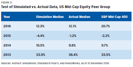
The authors highlighted that in 2016, both the actual and simulated results were far from the S&P Mid-Cap 400 return, while closer to the broader Russell Mid-Cap Index up 13.8% in 2016.
It illustrates to them another important point in using simulating peer group. A fund manager focusing primarily on beating the index takes a risk in straying outside the index constituents, as illustrated in 2016. Instead, if the fund manager focuses on stock selection from a broad universe (i.e., active fund managers with high off-benchmark ratio), a simulated peer group universe can provide the needed understanding and validation when the index fell to do so.
In conclusion
The approach described here is definitely helpful to judge a manager’s performance in the absence of a suitable peer group or index. It’s application, might however be difficult as it requires advanced statistical tools to run randomly simulated portfolios with constraints. Moreover, if you want to add sophisticated rebalancing rules to better replicate the manager’s risk management policies.
At WSP we have worked extensively on peer group building, and we are cognisant using peer group simulation is beneficial. We cross-check that approach with performance attribution analysis and risk factor analysis to reach to a robust in-depth understanding of the source of performance and to what extent it is attributable to true manager skills rather to a set of identified constraint biases.
To notice lastly, all the above analysis applied nicely to equity portfolios, but we believe less so for fixed income portfolios. To build a robust simulated peer group based on set of rules and constraints using a universe of bond made of a large number of, and ever changing, bonds presents true challenges still to be solved to our opinion.